Marek Oerlemans

Find out about my work
Exploring e-means, the faster brother of k-means
By Marek Oerlemans November 2026
Last week, e-means was published (Bessa et al., 2026): a new k-means algorithm that claims to reach the same clustering quality as the classic methods in about a tenth of the work. It comes with tuned hyperparameters, scaling laws, and one design choice that made me stop and squint. This post is about that choice: what I expected it to do, what it actually does, and what happens when you take it apart.
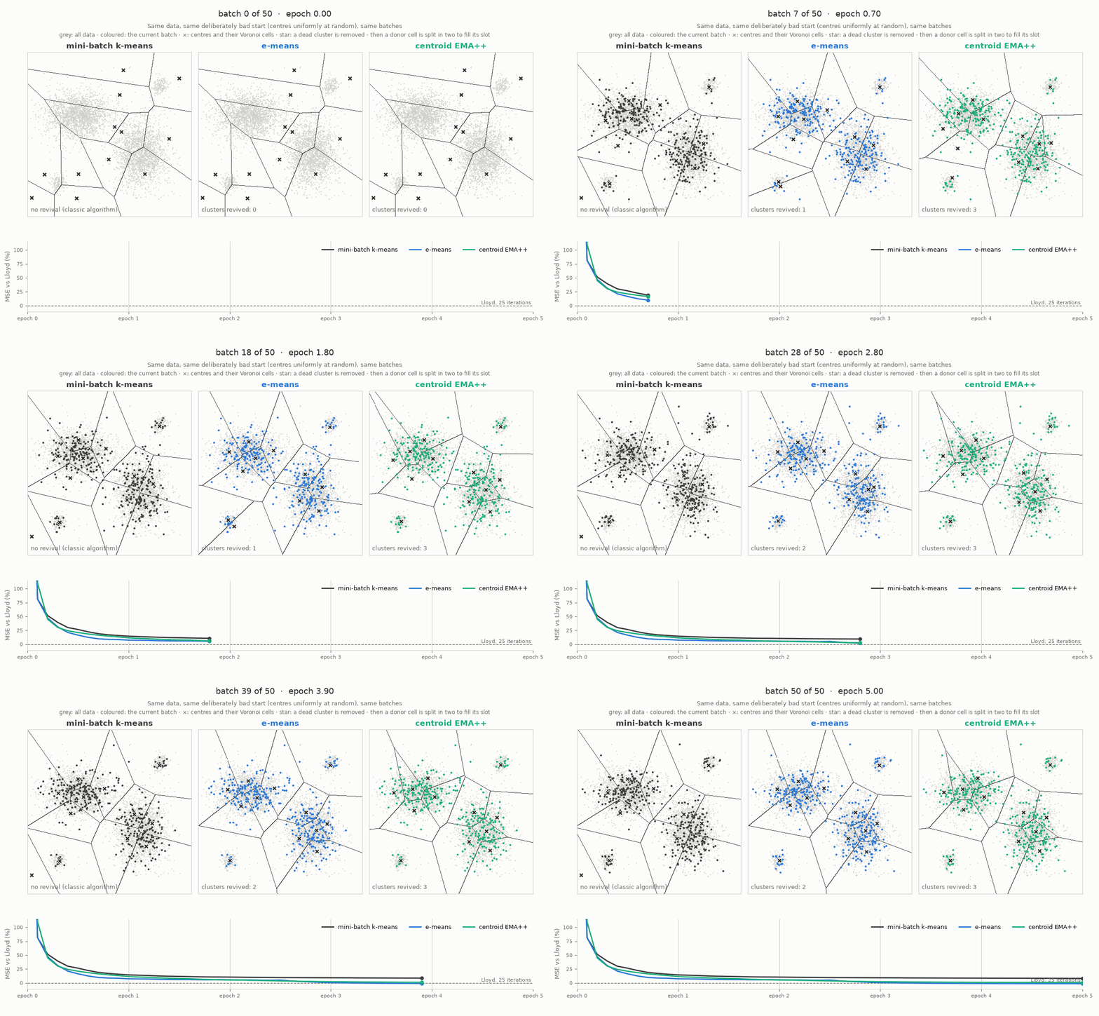
From Lloyd to e-means
The classic way to do k-means is Lloyd’s algorithm (Lloyd, 1982). It repeats two steps over the whole dataset: assign every point to its nearest cluster centre, then move every centre to the mean of its points. Every iteration is a full pass over the data, and you typically need a few dozen of them; 25 is the default in Faiss, and the paper’s yardstick. Flash-KMeans (Yang et al., 2026) recently made each pass much faster on a GPU, but you still need all those passes.
So why wait for the whole dataset before moving the centres? Take a small batch of points, assign them, nudge the centres a bit, and repeat. That’s mini-batch k-means (Sculley, 2010). In its classic form, every centre is the running mean of all points it has ever been given: it keeps a running sum and a running count, and its step is one over the number of points it has seen. Big steps at the start, smaller and smaller ones after that.
e-means is a mini-batch method too (the “e” presumably stands for exponential moving average; the paper never actually says). After every batch, each cluster $j$ that got $n_j$ points with sum $s_j$ updates two moving averages, one of the sum and one of the count:
\[N_j \leftarrow \gamma N_j + \alpha\, n_j, \qquad S_j \leftarrow \gamma S_j + \alpha\, s_j, \qquad c_j = S_j / N_j.\]Note what kind of objects these are. $S_j$ is a vector, a (moving) sum of points, with the same dimension as the data. $N_j$ is a single number, a (moving) count of points. The centre $c_j$ is just their ratio. And because $N_j$ is a moving average, it’s not a whole number: a cluster can have a count of 37.4. The step $\alpha = 1 - \gamma$ follows a cosine schedule, and the batch size and starting step come from the paper’s scaling laws.
Why keep a count at all?
Here’s what made me squint. The centre is the only thing you need for the next batch. So why carry around a sum and a count, and divide them every time? Why not just keep a moving average of the centres themselves?
\[c_j \leftarrow c_j + \alpha\,(m_j - c_j),\]with $m_j = s_j / n_j$ the mean of the points cluster $j$ got in this batch. Same idea, half the bookkeeping. I called it the centroid EMA.
(In hindsight, the sum and the count aren’t that exotic: classic mini-batch k-means keeps exactly those two, as running totals. e-means just lets them fade. But a count that isn’t a whole number still felt odd to me, so let’s see whether it’s needed.)
Before looking at the results: what would you expect? The two updates look like they should do the same thing.
The setup. SIFT-128 from ann-benchmarks: 200k vectors to cluster into $k = 2048$ clusters (about 100 points each), the 10k provided queries as test set, and 10k other vectors to tune on. Every method uses the paper’s scaling laws for its batch size and step, and gets 5 random seeds. All numbers in this post are the MSE on the test set. I look at each method two ways:
- During training: one 10-epoch run, measured after every epoch, like Lloyd’s curve.
- Per budget: a separate run for 1, 2, 3, 5 and 10 epochs, each with its own schedule. This is how the paper reports results: what you get if you know your budget in advance.
Everything is measured relative to 25 iterations of Lloyd.
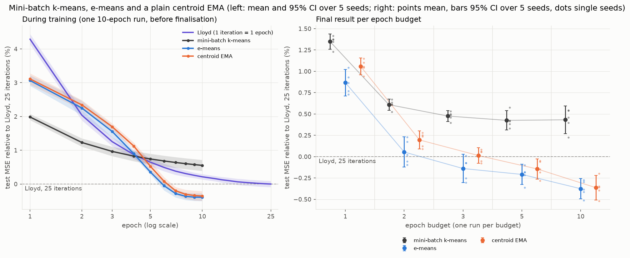
Figure 1. Left: test MSE during one 10-epoch run, with Lloyd’s curve per iteration; bands are 95% confidence intervals over 5 seeds. Right: the result per epoch budget; points are means with 95% confidence intervals, the small dots single seeds. Mini-batch k-means gets the same dead-cluster revival as e-means, so only the update differs.
First, the reproduction (right). We find the same as the paper: within 2 to 3 epochs, e-means reaches the result of 25 iterations of Lloyd, and it keeps improving after that.
Classic mini-batch k-means stalls at about 0.4% above Lloyd: as the paper already notes, forgetting old batches is what keeps e-means moving.
And my centroid EMA? During training it seems to behave a bit differently from e-means, trailing it through the middle epochs. But the final results per budget are quite similar.
So is the count really unnecessary, or is it doing something we don’t see in the final numbers? Let’s look at what it actually does.
What the count actually does
Let’s rewrite e-means’ update as a step of the centre, so we can compare it with the centroid EMA. Write the sum as count times centre, $S_j = N_j c_j$, and the same for the batch, $s_j = n_j m_j$. Then the new centre is
\[c_j' = \frac{\gamma S_j + \alpha s_j}{\gamma N_j + \alpha n_j} = \frac{\gamma N_j\, c_j + \alpha n_j\, m_j}{\gamma N_j + \alpha n_j}.\]That’s a weighted average of the old centre and the batch mean, which we can write as a step from the old centre towards the batch mean:
\[c_j' = c_j + a_j\,(m_j - c_j), \qquad a_j = \frac{\alpha\, n_j}{\gamma N_j + \alpha\, n_j}.\]So my centroid EMA is really just e-means with the step $a_j$ of every cluster fixed to $\alpha$. Stare at $a_j$ for a moment. It hides two things that my centroid EMA throws away.
1. The step depends on how many points the cluster got. Once things have settled, $N_j$ is about the number of points the cluster usually gets per batch; call it $\bar n_j$. For small $\alpha$ the step is then roughly
\[a_j \approx \alpha\, \frac{n_j}{\bar n_j}.\]A cluster that got its usual number of points moves $\alpha$. A cluster that got a single point barely moves on the basis of that one point; one that got twice its usual number moves about twice as far. My centroid EMA moves every cluster by the same $\alpha$, however little evidence it has.
2. It starts with a warm-up. This comes from how the count is initialised. Every centre starts at a random data point, and the count starts at $N_j = 10^{-10}$: basically zero, so the starting centre carries almost no weight. On a cluster’s first batch, $a_j \approx 1$, and the centre jumps all the way to the mean of its points. After that the count builds up. If a cluster gets the same $\bar n$ points every batch, the count after $t$ batches is $N_t = \bar n\,(1 - \gamma^t)$, and the step becomes
\[a_t = \frac{\alpha \bar n}{\gamma\, \bar n (1 - \gamma^{t-1}) + \alpha \bar n} = \frac{\alpha}{1 - \gamma^t}.\]That’s a step that starts at 1 and decays to $\alpha$ over roughly $1/\alpha$ batches. It’s the standard bias correction for a moving average that starts at zero: early on, the average is built from only a few batches, so you divide by the total weight it has seen so far, $1 - \gamma^t$. (With a schedule, $\gamma^t$ becomes the product of all $\gamma$’s so far.)
And the count has a third job, outside the update: reviving dead clusters. With random starting centres, quite a few clusters land in empty regions and never get any points. So every 5 batches, e-means checks every cluster’s count:
- A cluster is dead if its count has dropped below 10% of the average count, meaning it has hardly received any points for a while.
- For every dead cluster, a donor is drawn from the live clusters, with a chance proportional to its count, so busy clusters are the likely donors. Each donor is used at most once per check.
- The donor’s centre is split into two slightly perturbed copies. The donor keeps one copy; the other replaces the dead cluster. Both get half of the donor’s count and sum.
The idea: a busy cluster probably covers a region that deserves two centres, so the dead cluster’s slot is better spent there.
Three jobs for one number. Can we do the first two without it?
Centroid EMA+: the count without the count
One thing at a time: here we only change the update, and leave revival as it is. We’ll come back to revival in the next section.
Centroid EMA+ adds both missing pieces to the centroid EMA:
- A count-scaled step. Pretend every point is its own small EMA step. Then $n_j$ points move the centre a fraction $1 - (1 - \eta)^{n_j}$ of the way. Choose $\eta$ so that a cluster with an average number of points ($B/k$) moves exactly the scheduled $\alpha$, and you get $a_j = 1 - (1 - \alpha)^{n_j k / B}$. For small $\alpha$ this is about $\alpha\, n_j / (B/k)$: the same shape as e-means’ $\alpha\, n_j / \bar n_j$, and it never steps past the batch mean either. The difference is what it compares with: the average cluster instead of the cluster’s own history, so it needs no count per cluster.
- A warm-up. Use the bias-corrected step from above, $\alpha / (1 - \prod \gamma)$. Since it doesn’t depend on the cluster, it’s one number for all clusters.
So, let’s see how the centroid EMA does with these better steps.
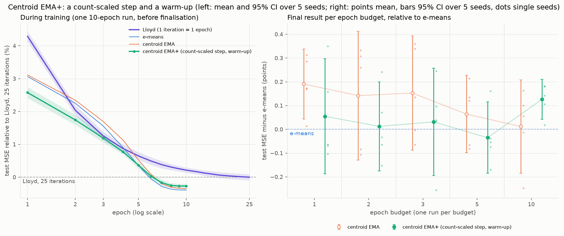
Figure 2. Left: during training. Right: result per budget, relative to e-means at the same budget and seed. Hollow: the plain centroid EMA from figure 1.
It works. Centroid EMA+ is about level with e-means at every budget, and during training it’s even ahead in the first epochs.
Neither piece does it alone. At 1 epoch, the warm-up alone doesn’t help and the scaled step alone makes things worse; only together do they close the gap. From 3 epochs on, the scaled step does most of the work. And at the shortest budget the step size matters just as much: the scaling laws were tuned for e-means, and our variants would like a step about 1.4 times bigger.
That leaves the third job. Centroid EMA+ still keeps a count, only for revival. Can we get rid of it there too?
Getting rid of the count
First, how much does revival matter? Let’s switch it off, for e-means, for centroid EMA+, and for classic mini-batch k-means.
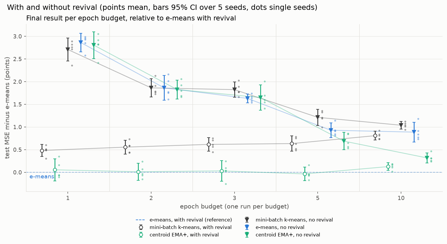
Figure 3. Result per budget with revival (hollow circles) and without (triangles), relative to e-means with revival.
Revival matters a lot, for all three methods, as the paper also finds. The effect gets smaller the longer you train, but even at 10 epochs it hasn’t gone away.
The culprit is the random start. Many starting centres land in empty regions and never get a single point. Without revival they stay dead: after 3 epochs, one in six to one in eight clusters is still (almost) empty, for all three methods. With revival, that repair happens almost entirely in the first epoch: of the 350 to 850 clusters revived in a 3-epoch run, at most 25 are revived later.
So all three methods need revival, and revival needs the count. Can we find something else that tells us a cluster is dead?
What does a dead cluster look like, besides having no points? It contributes nothing to the error. So instead of the count, we track a moving average of each cluster’s error, the sum of squared distances of its points in the batch to its centre:
\[E_j \leftarrow \gamma E_j + \alpha\, e_j, \qquad e_j = \sum_{x \in \text{batch},\ x \to j} \lVert x - c_j \rVert^2.\]We compute those distances anyway during the assignment, so it’s free. A cluster that stops getting points sees its error fade to zero. The new rule:
- Dead: a cluster whose error has dropped below 10% of the average error.
- Donor: drawn from the live clusters with a chance proportional to their error, so the clusters that contribute most to the error get split. Each donor is used at most once per check.
- Split: as before. The donor’s centre is split into two slightly perturbed copies; the donor keeps one, the dead cluster gets the other, and both get half the donor’s error.
- When: every batch instead of every 5. The error is updated every batch anyway, and with the count rule checking every batch made no clear difference, so from here on both rules check every batch.
That’s centroid EMA++: per cluster just a centre and an error. No sums, no counts.
So we have two updates (e-means and centroid EMA+) and two revival rules (count and error). Let’s compare all four combinations.
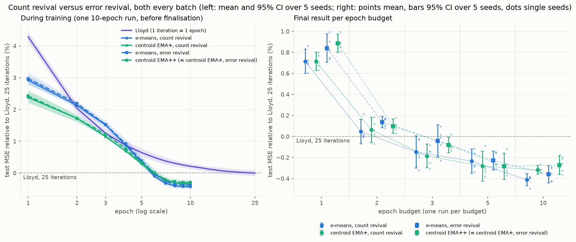
Figure 4. e-means (blue) and centroid EMA+ (green), each with count revival (circles, solid) and error revival (squares, dashed), all checking every batch. Left: during training. Right: result per budget, relative to Lloyd.
The error does the job. All four end up in the same place. The error rule is slightly worse than the count at 1 epoch, and about the same after that.
Which clusters actually get killed? Mostly the ones that started dead: nearly all revivals happen in the first epoch, where they repair the random start. But the two rules don’t flag exactly the same clusters. Nearly every cluster that’s dead by error is also dead by count, but the count flags more. After the first epoch, only about half of the clusters the count rule would revive are dead by error too. And the error rule occasionally revives a cluster that still has points but almost no error: a very tight cluster that the count would have left alone. Only partial overlap, but the same end result.
Cost-wise nothing changes. Assigning a batch takes $O(Bkd)$, which dwarfs the $O(k)$ check for dead clusters, even every batch; and the error comes for free with distances we already have. Every method keeps one vector and one number per cluster.
So what?
e-means combines two moving averages, one of a sum and one of a count. My first reaction: that’s unnatural. A count that isn’t a whole number gives me the ick, so I tried to remove it.
It turns out the count does more than you’d see at face value: it scales each cluster’s step by how much evidence the cluster has, it gives every cluster a warm-up from its near-zero start, and it finds dead clusters.
Make those three jobs explicit and you get a reparametrisation of the paper’s algorithm: a centroid EMA with a count-scaled step, a warm-up and error-based revival. It still works: it performs about the same and costs the same in memory and compute. It was a great way to understand the paper, and to follow my own first thoughts when I saw it.
This was a small weekend exploration on one small dataset (200k SIFT vectors), not a benchmark: the differences are tiny, and I wouldn’t bet on any of them carrying over to the billion-point problems in the paper. Code and all numbers are on GitHub.
References
- Bessa et al. (2026). e-means: outperforming k-means (in one-tenth the epochs). arXiv:2611.09501.
- Lloyd, S. P. (1982). Least squares quantization in PCM. IEEE Transactions on Information Theory 28(2).
- Sculley, D. (2010). Web-scale k-means clustering. WWW 2010.
- Yang, S. et al. (2026). Flash-KMeans: fast and memory-efficient exact K-means. arXiv:2603.09229.